When we’re dealing with big amounts of data, each point in the data set gives us varying information about the final outcome. That means there is always some impurity in our data. This impurity can be quantified by calculating the entropy of the given data. On the other hand, each data point gives differing information on the final outcome. Information gain indicates how much information a given variable/feature gives us about the final outcome. Before we explain more in-depth about entropy and information gain, we need to become familiar with a powerful tool in the decision making universe: decision trees.
1. What is a decision tree?
A decision tree is just a flow chart like structure that helps us make decisions. Below is a simple example of a decision tree.
As we can see, a decision tree allows us to follow a certain path to arrive at a conclusion. While programming, the yes and no could be simple if-else conditions. We split our data into subsets based on some variable (eg: gender, age) which we can use to develop a decision tree so our program knows what to do with our data. We’ll talk more in detail down the line.
2. Entropy
The real-world definition of the term entropy might be familiar to one. Let’s take a look at it.
A thermodynamic quantity representing the unavailability of a system's thermal energy for conversion into mechanical work, often interpreted as the degree of disorder or randomness in the system
If one doesn’t understand it or even if one does, it’s totally fine. In simple terms, entropy is the degree of disorder or randomness in the system. In data science, entropy pretty much refers to the same. The degree of randomness in a data set will indicate how impure or uncertain the data in the set is. The entropy of the whole set of data can be calculated by using the following equation.
S - Set of all instances
N - Number of distinct class values
Pi - Event probablity
For those not coming from a physics/probability background, the above equation could be confusing. But do not worry. We will discuss it in-depth as we go down.
3. Information gain (IG)
As already mentioned, information gain indicates how much information a particular variable or feature gives us about the final outcome. It can be found out by subtracting the entropy of a particular attribute inside the data set from the entropy of the whole data set.
H(S) - entropy of whole data set S
|Sj| - number of instances with j value of an attribute A
|S| - total number of instances in the dataset
v - set of distinct values of an attribute A
H(Sj) - entropy of subset of instances for attribute A
H(A, S) - entropy of an attribute A
There will be some difficulty in understanding the terms and logic behind the equation. The idea is simple. We reduce the entropy of the subset having attribute A from the entropy of the whole set S. The difference will give us the amount of information we have gained. Again, one shall understand as we go down.
4. A use case for entropy and information gain
Trying to understand entropy and information gain in plain theory is a bit difficult. It is best understood via an example. Let’s look at the following problem statement.
There is an international series going on between India and England. The match will happen if the weather conditions are okay. Otherwise, the match will be suspended. Now forecast whether the match will happen or not depending on the weather condition.
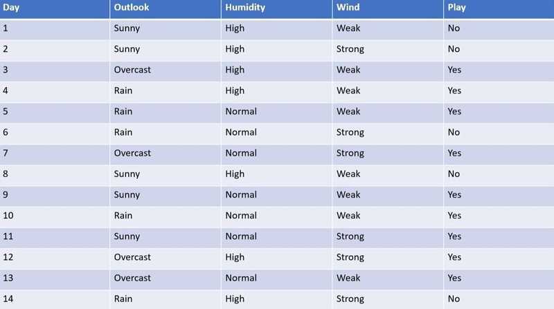
Here the predictor variables are outlook, humidity, and wind while the target variable is play. Hence, if the combination of outlook, humidity, and the wind is right, we can play. Otherwise, the match will not happen. In order to make this possible, we have to make a decision tree.
For a decision tree to be made, we first need a root variable. Because a decision tree, as already exemplified above starts with a root node. Here three variables - outlook, humidity, and wind determines the final outcome. While all three variables play an important role in the final outcome, one of them will play the most important role. Now let’s quote something we already talked about above.
...information gain indicates how much information a particular variable or feature gives us about the final outcome.
So, in order to find our root node, we have to calculate the information gain of each of our variables. The variable with the highest information gain will be the most important variable and hence our root variable.
To calculate information gain, we need to first calculate entropy. Let’s revisit entropy’s equation.
Here N is the number of distinct class values. The final outcome is either yes or no. So the number of distinct class values is 2.
Pi is the probability of the event. There are 2 events as outcomes here, as already mentioned above. One is the event “yes” and the other is the event “no”. In a total of 14, 9 cases are Yes and the rest 5 cases, the outcome is No.
So Yes (P1) has a probability of 9/14 while No (P2) has a probability of 5/14.
Now what is remaining is only applying these values to the above equation.
Hence entropy of our data set is 0.940.
4.1 Information Gain
Now it is time to calculate the IG of each variable. Let’s recap the formula once again.
4.2 IG of outlook
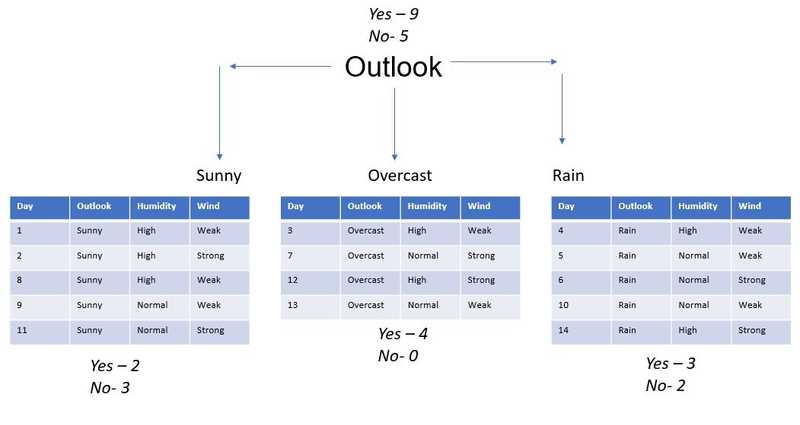
Outlook can have 3 values which is Sunny, Overcast, and Rainy. Hence v will be 3. Outlook has 5 instances that have the value “Sunny”, 4 instances that have the value “Overcast”, and 5 instances that have the value “Rainy”. Hence the 3 values of Sj/S will be 5/14, 4/14, and 5/14.
H(Sj) represents the entropy of that particular instance.
Out of 5 instances which is Sunny, 2 are playable. Hence 2/5.
Out of 4 instances which is Overcast, all 4 are playable. Hence 4/4.
Out of 5 instances which is Rainy, 3 are playable. Hence 3/5.
Now let’s substitute the values into the equation.
Hence the gain of outlook is 0.247.
4.3 IG of wind
Wind can have 2 values which are weak and strong. Hence v will be 2. Wind has 8 instances which has value “weak” and 6 instances which has value “strong”. Hence the 2 values of Sj/S will be 8/14 and 6/14.
H(Sj) represents the entropy of that particular instance.
Out of 8 instances which is Weak, 6 are playable. Hence 6/8.
Out of 6 instances which is Strong, 3 are playable. Hence 3/6.
Now let’s substitute the values into the equation.
Hence the gain of Wind is 0.048.
4.4 IG of humidity
Humidity can have 2 values which are high and normal. Hence v will be 2. Humidity has 7 instances which has value “high” and 7 instances which has value “normal”. Hence the 2 values of Sj/S will be 7/14 and 7/14.
H(Sj) represents the entropy of that particular instance.
Out of 7 instances which is high, 3 are playable. Hence 3/7.
Out of 7 instances which is normal, 6 are playable. Hence 6/7.
Now let’s substitute the values into the equation.
Hence the gain of Humidity is 0.151.
Here the variable Outlook has the highest gain (0.247) hence should be taken as the root variable. If we just scan over the table above, it should be obvious that the outlook variable has the most effect on the final outcome. However, when we are dealing with actual data science projects, the data will be big and complex. Hence it is easier to find the gain of variables and use the variable with the highest gain as the root.
4.5 Decision Tree
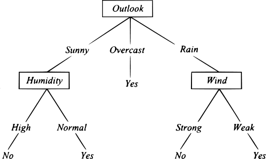
Now that we have our root variable, we can finally make our decision tree.
Since the outlook variable has the most importance to the final outcome, it makes sense to start our decision tree with outlook. This is a very simple example. But when we’re going to be dealing with huge and complex data, having the most consequential variable as our root is important for efficiency. Just taking a look at the decision tree, we can see that if the value of the variable outlook is overcast, we don’t even have to check other variable values. The final outcome is already yes. One can guess how this improves the efficiency of our program. This is especially true when writing decision tree algorithms for machine learning. We have to follow a pattern in which the most important variable is checked first and the least important one is checked last. For that, we must calculate the information gain of all the variables and write our algorithm accordingly.


